|
Figure 1: Single segment storage allocation
bunch of segments all starting at zero are relocated one after another |
|
A linker or loader's first major task is storage allocation. Once storage is allocated, the linker can proceed to subsequent phases of symbol binding and code fixups. Most of the symbols defined in a linkable object file are defined relative to storage areas within the file, so the symbols cannot be resolved until the areas' addresses are known.
As is the case with most other aspects of linking, the basic issues in storage allocation are straightforward, but the details to handle peculiarities of computer architecture and programming language semantics (and the interactions between the two) can get complicated. Most of the job of storage allocation can be handled in an elegant and relatively architecture-independent way, but there are invariably a few details that require ad hoc machine specific hackery. |
Each of the linker's input files contains a set of segments of various types. Different kinds of segments are treated in different ways. Most commonly all segments of a particular type. such as executable code, are concatenated into a single segment in the output file. Sometimes segments are merged one on top of another, as for Fortran common blocks, and in an increasing number of cases, for shared libraries and C++ special features, the linker itself needs to create some segments and lay them out.
Storage layout is a two-pass process, since the location of each segment can't be assigned until the sizes of all segments that logically precede it are known.
|
|
Figure 1: Single segment storage allocation
bunch of segments all starting at zero are relocated one after another |
The linker or loader examines each module in turn, allocating storage sequentially. The starting address of Mi is the sum of L1 through Li-1, and the length of the linked program is the sum of L1 through Ln.
Most architectures require that data be aligned on word boundaries, or at least run faster if data is aligned, so linkers generally round each Li up to a multiple of the most stringent alignment that the architecture requires, typically 4 or 8 bytes.
Example 1: Assume a main program called main is to be linked with three subroutines called calif, mass, and newyork. (It allocates venture capital geographically.) The sizes of each routine are (in hex): l r. name size _ main 1017 calif 920 mass 615 newyork 1390 Assume that storage allocation starts at location 1000 hex, and that the alignment is four bytes. Then the allocations might be: l r. name location _ main 1000 - 2016 calif 2018 - 2937 mass 2938 - 2f4c newyork 2f50 - 42df Due to alignment, one byte at 2017 and three bytes at 2f4d are wasted, not enough to worry about.
|
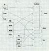
In all but the simplest object formats, there are several kinds of segment, and the linker needs to group corresponding segments from all of the input modules together. On a Unix system with text and data segments, the linked file needs to have all of the text collected together, followed by all of the data, followed logically by the BSS. (Even though the BSS doesn't take space in the output file, it needs to have space allocated to resolve BSS symbols, and to indicate the size of BSS to allocate when the output file is loaded.) This requires a two-level storage allocation strategy.
Now each module Mi has text size Ti, data size Di, and BSS size Bi, Figure 2.
As it reads each input module, the linker allocates space for each of the Ti, Di, and Bi as though each segment were separately allocated at zero. After reading all of the input files, the linker now knows the total size of each of the three segments, Ttot, Dtot, and Btot. Since the data segment follows the text segment, the linker adds Ttot to the address assigned for each of the data segments, and since the BSS segment follows both the text and data segments, the linker adds the sum of Ttot and Dtot to the allocated BSS segments.
Again, the linker usually needs to round up each allocated size.
Segment and page alignmentIf the text and data segments are loaded into separate memory pages, as is generally the case, the size of the text segment has to be rounded up to a full page and the data and BSS segment locations correspondingly adjusted. Many Unix systems use a trick that saves file space by starting the data immediately after the text in the object file, and mapping that page in the file into virtual memory twice, once read-only for the text and once copy-on-write for the data. In that case, the data addresses logically start exactly one page beyond the end of the text, so rather than rounding up, the data addresses start exactly 4K or whatever the page size is beyond the end of the text.
|
The linker first lays out the text, then the data, then the bss. Note that the data section starts on a page boundary at 0x5000, but the bss starts immediately after the data, since at run time data and bss are logically one segment. l r r r. name text data bss _ main 1000 - 2016 5000 - 531f 695c - 69ab calif 2018 - 2937 5320 - 5446 69ac - 6aab mass 2938 - 2f4c 5448 - 5747 6aac - 72eb newyork 2f50 - 42df 5748 - 695a 72ec - 86eb There's wasted space at the end of the page between 42e0 and 5000. The bss segment ends in mid-page at 86eb, but typically programs allocate heap space starting immediately after that.
For the first 40 years of its existence, Fortran didn't support dynamic storage allocation, and common blocks were the primary tool that Fortran programmers used to circumvent that restriction. Standard Fortran permits blank common to be declared with different sizes in different routines, with the largest size taking precedence. Fortran systems universally extend this to allow all common blocks to be declared with different sizes, again with the largest size taking precedence.
Large Fortran programs often bump up against the memory limits in the systems in which they run, so in the absence of dynamic memory allocation, programmers frequently rebuild a package, tweaking the sizes to fit whatever problem a package is working on. All but one of the subprograms in a package declare each common block as a one-element array. One of the subprograms declares the actual size of all the common blocks, and at startup time puts the sizes in variables (in yet another common block) that the rest of the package can use. This makes it possible to adjust the size of the blocks by changing and recompiling a single routine that defines them, and then relinking.
As an added complication, starting in the 1960s Fortran added BLOCK DATA to specify static initial data values for all or part of any common block (except for blank common, a restriction rarely enforced.) Usually the size of the common block in the BLOCK DATA that initializes a block is taken to be the block's actual size at link time.
To handle common blocks, the linker treats the declaration of a common block in an input file as a segment, but overlays all of the blocks with the same name rather than concatenating these segments. It uses the largest declared size as the segment's size, unless one of the input files has an initialized version of the segment. In some systems, initialized common is a separate segment type, while in others it's just part of the data segment.
Unix linkers have always supported common blocks, since even the earliest versions of Unix had a Fortran subset compiler, and Unix versions of C have traditionally treated uninitialized global variables much like common blocks. But the pre-ELF versions of Unix object files only had the text, data, and bss segments with no direct way to declare a common block. As a special case hack, linkers treated a symbol that was flagged as undefined but nonetheless had a non-zero value as a common block, with the value being the size of the block. The linker took the largest value encountered for such symbols as the size of the common block. For each block, it defined the symbol in the bss segment of the output file, allocating the required amount of space after each symbol, Figure 3.
|
Figure 3: Unix common blocks
common at the end of bss |
In an environment in which each source file is separately compiled, a straightforward technique is to place in each object file all of the vtbls, expanded template routines, and extern inlines used in that file, resulting in a great deal of duplicated code.
The simplest approach at link time is to live with the duplication. The resulting program works correctly, but the code bloat can bulk up the object program to three times or more the size that it should be.
In systems stuck with simple-minded linkers, some C++ systems have used an iterative linking approach, separate databases of what's expanded where, or added pragmas (source code hints to the compiler) that feed back enough information to the compiler to generate just the code that's needed. We cover these in Chapter 11.
Many recent C++ systems have addressed the problem head-on, either by making the linker smarter, or by integrating the linker with other parts of the program development system. (We also touch on the latter approach in chapter 11.) The linker approach has the compiler generate all of the possibly duplicate code in each object file, with the linker identifying and discarding duplicates.
MS Windows linkers define a COMDAT flag for code sections that tells the linker to discard all but one identically named sections. The compiler gives the section the name of the template, suitably mangled to include the argument types, Figure 4
|
Figure 4: Windows
IMAGE_COMDAT_SELECT_NODUPLICATES 1 Warn if multiple identically named sections occur. IMAGE_COMDAT_SELECT_ANY 2 Link one identically named section, discard the rest. IMAGE_COMDAT_SELECT_SAME_SIZE 3 Link one identically named section, discard the rest. Warn if a discarded section isn't the same size. IMAGE_COMDAT_SELECT_EXACT_MATCH 4 Link one identically named section, discard the rest. Warn if a discarded section isn't identical in size and contents. (Not implemented.) IMAGE_COMDAT_SELECT_ASSOCIATIVE 5 Link this section if another specified section is also linked. |
The GNU linker deals with the template problem by defining a "link once" type of section similar to common blocks. If the linker sees segments with names of the form .gnu.linkonce.name it throws away all but the first such segment with identical names. Again, compilers expand a template to a .gnu.linkonce section with the name including the mangled template name.
This scheme works pretty well, but it's not a panacea. For one thing, it doesn't protect against the vtbls and expanded templates not actually being functionally identical. Some linkers attempt to check that the discarded segments are byte-for-byte identical to the one that's kept. This is very conservative, but can produce false errors if two files were compiled with different optimization options or with different versions of the compiler. For another, it doesn't discard nearly as much duplicated code as it could. In most C++ systems, all pointers have the same internal representation. This means that a template instantiated with, say, a pointer to int type and the same template instatiated with pointer to float will often generate identical code even though the C++ types are different. Some linkers may attempt to discard link-once sections which contain identical code to another section, even when the names don't quite match perfectly, but this issue remains unsatisfactorily resolved.
Although we've been discussing templates up to this point, exactly the same issues apply to extern inline functions and default constructor, copy, and assignment routines, which can be handled the same way.
The usual approach is for each object file to put any startup code into an anonymous routine, and to put a pointer to that routine into a segment called .init or something similar. The linker concatenates all the .init segments together, thereby creating a list of pointers to all the startup routines. The program's startup stub need only run down the list and call all the routines. Exit time code can be handled in much the same way, with a segment called .fini.
It turns out that this approach is not altogether satisfactory, because some startup code needs to be run earlier than others. The definition of C++ states that application-level constructors are run in an unpredictable order, but the I/O and other system library constructors need to be run before constructors in C++ applications are called. The ``perfect'' approach would be for each init routine to list its dependencies explicitly and do a topological sort. The BeOS dynamic linker does approximately that, using library reference dependencies. (If library A depends on library B, library B's initializers probably need to run first.)
A much simpler approximation is to have several initialization segments, .init and .ctor, so the startup stub first calls the .init routines for library-level initialization and then the .ctor routines for C++ constructors. The same problem occurs at the end of the program, with the corresponding segments being .dtor and .fini. One system goes so far as to allow the programmer to assign priority numbers, 0 to 127 for user code and 128-255 for system library code, and the linker sorts the initializer and finalizer routines by priority before combining them so highest priority initializers run first. This is still not altogether satisfactory, since constructors can have order dependencies on each other that cause hard-to-find bugs, but at this point C++ makes it the programmer's responsibility to prevent those dependencies.
A variant on this scheme puts the actual initialization code in the .init segment. When the linker combined them the segment would be in-line code to do all of the initializations. A few systems have tried that, but it's hard to make it work on computers without direct addressing, since the chunk of code from each object file needs to be able to address the data for its own file, usually needing registers that point to tables of address data. The anonymous routines set up their addressing the same way any other routine does, reducing the addressing problem to one that's already solved.
A related problem is that OS/360 didn't provide any support for what's now called per-process or task local storage, and very limited support for shared libraries. If two jobs ran the same program, either the program was marked reentrant, in which case they shared the entire program, code and data, or not reentrant, in which case they shared nothing. All programs were loaded into the same address space, so multiple instances of the same program had to make their arrangements for instance-specific data. (System 360s didn't have hardware memory relocation, and although 370s did, it wasn't until after several revisions of the OS/VS operating system that the system provided per-process address spaces.)
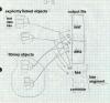
Pseudo-registers help solve both of these problems, Figure 5. Each input file can declare pseudo-registers, also called external dummy sections. (A dummy section in 360 assembler is analogous to a structure declaration.) Each pseudo-register has a name, length, and alignment. At link time, the linker collects all of the pseudo-registers into one logical segment, taking the largest size and most restrictive assignment for each, and assigns them all non-overlapping offsets in this logical segment.
But the linker doesn't allocate space for the pseudo-register segment. It merely calculates the size of the segment, and stores it in the program's data at a location marked by a special CXD, cumulative external dummy, relocation item. To refer to a particular pseudo-register, program code uses yet another special XD, external dummy, relocation type to indicate where to place the offset in the logical segment of one of the pseudo-registers.
The program's initialization code dynamically allocates space for the pseudo-registers, using a CXD to know how much space is needed, and conventionally places the address of that region in register 12, which remains unchanged for the duration of the program. Any part of the program can get the address of a pseudo-register by adding the contents of R12 to an XD item for that register. The usual way to do this is with a load or store instruction, using R12 as the index register and and XD item embedded as the address displacement field in the instruction. (The displacement field is only 12 bits, but the XD item leaves the high four bits of the 16-bit halfword zero, meaning base register zero, which produces the correct result.)
|
Figure 5: Pseudo-registers
bunch of chunks of space pointed to by R12. various routines offsetting to them |
The result of all this is that all parts of the program have direct access to all the pseudo-registers using load, store, and other RX format instructions. If multiple instances of a program are active, each instance allocates a separate space with a different R12 value.
Although the original motivation for pseudo-registers is now largely obsolete, the idea of providing linker support for efficient access to thread-local data is a good one, and has appeared in various forms in more modern systems, notably Windows32. Also, modern RISC machines share the 360's limited addressing range, and require tables of memory pointers to address arbitrary memory locations. On many RISC UNIX systems, a compiler creates two data segments in each module, one for regular data and one for "small" data, static objects below some threshold size. The linker collects all of the small data segments together, and arranges for program startup code to put the address of the combined small data segment in a reserved register. This permits direct references to small data using based addressing relative to that register. Note that unlike pseudo-registers, the small data storage is both laid out and allocated by the linker, and there's only one copy of the small data per process. Some UNIX systems support threads, but per-thread storage is handled by explicit program code without any special help from the linker.
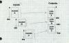
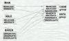
Figure 6 shows a program linked from three input files, main, able, and baker. Main contains segments MAINCODE and MAINDATA, able contains ABLECODE, and ABLEDATA, and baker contains BAKERCODE, BAKERDATA, and BAKERLDATA. Each of the code sections in in the CODE class and the data sections are in the DATA class, but the BAKERLDATA "large data" section is not assigned to a class. In the linked program, assuming the CODE sections are a total of 64K or less, they can be treated as a single segment at runtime, using short rather than long call and jump instructions and a single unchanging CS code segment register. Likewise, if all the DATA fit in 64K they can be treated as a single segment using short memory reference instructions and a single unchanging DS data segment register. The BAKERLDATA segment is handled at runtime as a separate segment, with code loading a segment register (usually the ES) to refer to it.
|
Figure 6: X86
CODE class with MAINCODE, ABLECODE, BAKERCODE DATA class with MAINDATA, ABLEDATA, BAKERDATA BAKERLDATA |
Real mode and 286 protected mode programs are linked almost identically. The primary difference is that once the linker creates the linked segments in a protected mode program, the linker is done, leaving the actual assignment of memory locations and segment numbers until the program is loaded. In real mode, the linker has an extra step that allocates the segments to linear addresses and assigns "paragraph" numbers to the segments relative to the beginning of the program. Then at load time, the program loader has to fix up all of the paragraph numbers in a real mode program or segment numbers in a protected mode program to refer to the actual location where the program is loaded.
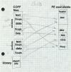
Other linkers have defined a script language to control the linker's output. The GNU linker, which also has a long list of command line switches, defines such a language. Figure 7 shows a simple linker script that produces COFF executables for System V Release 3.2 systems such as SCO Unix.
|
Figure 7: GNU linker control script for COFF executable
|
The first few lines describe the output format, which must be present in a table of formats compiled into the linker, the place to look for object code libraries, and the name of the default entry point, _start in this case. Then it lists the sections in the output file. An optional value after the section name says where the section starts, hence the .text section starts immediately after the file headers. The .text section in the output file contains the .init sections from all of the input files, then the .text sections, then the .fini sections. The linker defines the symbol etext to be the address after the .fini sections. Then the script sets the origin of the .data section, to start on a 4K page boundary roughly 400000 hex beyond the end of the text, and the section includes the .data sections from all the input files, with the symbol edata defined after them. Then the .bss section starts right after the data and includes the input .bss sections as well as any common blocks with end marking the end of the bss. (COMMON is a keyword in the script language.) After that are two sections for symbol table entries collected from the corresponding parts of the input files, but not loaded at runtime, since only a debugger looks at those symbols. The linker script language is considerably more flexible than this simple example shows, and is adequate to describe everything from simple DOS executables to Windows PE executables to complex overlaid arrangements.
Linkers for specialized processors like DSPs have special features to support the peculiarities of each processor. For example, the Motorola 5600X DSPs have support for circular buffers that have to be aligned at an address that is a power of two at least as large as the buffer. The 56K object format has a special segment type for these buffers, and the linker automatically allocates them on a correct boundary, shuffling segments to minimize unused space.
|
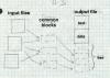
Figure 8: a.out linking
picture of text, data, and bss/common from explicit and library objects being combined into three big segments |
At this point, the linker can assign addresses to all of the segments. The text segment starts at a fixed location that depends on the variety of a.out being created, either location zero (the oldest formats), one page past location zero (NMAGIC formats), or one page plus the size of the a.out header (QMAGIC.) The data segment starts right after the data segment (old unshared a.out), on the next page boundary after the text segment (NMAGIC). In every format, bss starts immediately after the data segment. Within each segment, the linker allocates the segments from each input file starting at the next word boundary after the previous segment.

|
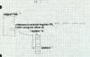
Figure 9: ELF linking
Adapt figs from pages 2-7 and 2-8 of TIS ELF doc show input sections turning into output segments. |
ELF objects have the traditional text, data, and bss sections, now spelled .text, .data, and .bss. They also often contain .init and .fini, for startup and exit time code, as well as various odds and ends. The .rodata and .data1 sections are used in some compilers for read-only data and out-of-line data literals. (Some also have .rodata1 for out-of-line read-only data.) On RISCsystems like MIPS with limited sized address offsets, .sbss and .scommon, are "small" bss and common blocks to help group small objects into one directly addressable area, as we noted above in the discussion of pseudo-registers. On GNU C++ systems, there may also be linkonce sections to be included into text, rodata, and data segments.
Despite the profusion of section types, the linking process remains about the same. The linker collects each type of section from the input files together, along with sections from library objects. The linker also notes which symbols will be resolved at runtime from shared libraries, and creates .interp, .got, .plt, and symbol table sections to support runtime linking. (We defer discussion of the details until Chapter 9.) Once that is all done, the linker allocates space in a conventional order. Unlike a.out, ELF objects are not loaded anywhere near address zero, but are instead loaded in about the middle of the address space so the stack can grow down below the text segment and the heap up from the end of the data, keeping the total address space in use relative compact. On 386 systems, the text base address is 0x08048000, which permits a reasonably large stack below the text while still staying above address 0x08000000, permitting most programs to use a single second-level page table. (Recall that on the 386, each second-level table maps 0x00400000 addresses.) ELF uses the QMAGIC trick of including the header in the text segment, so the actual text segment starts after the ELF header and program header table, typically at file offset 0x100. Then it allocates into the text segment .interp (the logical link to the dynamic linker, which needs to run first), the dynamic linker symbol table sections, .init, the .text and link-once text, and the read-only data.
Next comes the data segment, which logically starts one page past the end of the text segment, since at runtime the page is mapped in as both the last page of text and the first page of data. The linker allocates the various .data and link-once data, the .got section and on platforms that use it, .sdata small data and the .got global offset table.
Finally come the bss sections, logically right after the data, starting with .sbss (if any, to put it next to .sdata and .got), the bss segments, and common blocks.
|
Figure 10: PE storage allocation
adapt from MS web site |
PE executable files are conventionally loaded at 0x400000, which is where the text starts. The text section includes text from the input files, as well as initialize and finalize sections. Next comes the data sections, aligned on a logical disk block boundary. (Disk blocks are usually smaller than memory pages, 512 or 1K rather than 4K on Windows machines.) Following that are bss and common, .rdata relocation fixups (for DLL libraries that often can't be loaded at the expected target address), import and export tables for dynamic linking, and other sections such as Windows resources.
An unusual section type is .tls, thread local storage. A Windows process can and usually does have multiple threads of control simultaneously active. The .tls data in a PE file is allocated for each thread. It includes both a block of data to initialize and an array of functions to call on thread startup and shutdown.
1. Why does a linker shuffle around segments to put segments of the same type next to each other? Wouldn't it be easier to leave them in the original order?
2. When, if ever, does it matter in what order a linker allocates storage for routines? In our example, what difference would it make if the linker allocated newyork, mass, calif, main rather than main, calif, mass, newyork. (We'll ask this question again later when we discuss overlays and dynamic linking, so you can disregard those considerations.)
3. In most cases a linker allocates similar sections sequentialy, for example, the text of calif, mass, and newyork one after another. But it allocates all common sections with the same name on top of each other. Why?
4. Is it a good idea to permit common blocks declared in different input files with the same name but different sizes? Why or why not?
5. In example 1, assume that the programmer has rewritten the calif routine so that the object code is now hex 1333 long. Recompute the assigned segment locations. In example 2, further assume that the data and bss sizes for the rewritten calif routine are 975 and 120. Recompute the assigned segment locations.
Project 4-2: Implement Unix-style common blocks. That is, scan the symbol table for undefined symbols with non-zero values, and add space of appropriate size to the .bss segment. Don't worry about adjusting the symbol table entries, that's in the next chapter.
Project 4-3: Extend the allocator in 4-3 to handle arbitrary segments in input files, combining all segments with identical names. A reasonable allocation strategy would be to put at 1000 the segments with RP attributes, then starting at the next 1000 boundary RWP attributes, then on a 4 boundary RW attributes. Allocate common blocks in .bss with attribute RW.